Module 1: Data Import & Quality Control
Understanding your genomic data
Why Genomics in Plant Breeding?
Before we dive into the software, let’s understand why we’re doing this.
The Traditional Breeding Challenge
Plant breeders have always faced the same problem: you can’t see genes. Historically, breeders had to:
- Make crosses
- Grow plants to maturity
- Measure traits (yield, disease resistance, etc.)
- Select the best individuals
- Repeat for many generations
This works, but it’s slow and expensive — especially for traits that take years to measure (like tree fruit quality) or require destroying the plant (like root characteristics).
What Genomic Data Gives Us
With genomic markers (SNPs), we can:
- See inside the genome — Identify which genetic variants each individual carries
- Predict performance — Estimate breeding value before measuring the trait
- Select earlier — Make decisions at the seedling stage
- Understand relationships — See how individuals are related genetically
Genomic data lets us make better breeding decisions, faster.
What is a SNP?
A SNP (Single Nucleotide Polymorphism) is a position in the genome where individuals differ by a single DNA base.
Individual 1: ...ATCGATCG[A]TCGATCG...
Individual 2: ...ATCGATCG[G]TCGATCG...
                          ^
                         SNP
When we “genotype” plants, we’re measuring thousands of these SNPs across the genome. This gives us a genomic fingerprint for each individual.
Getting Started with BIGapp
Open BIGapp
Go to: big-demo.shinyapps.io/bigapp-main
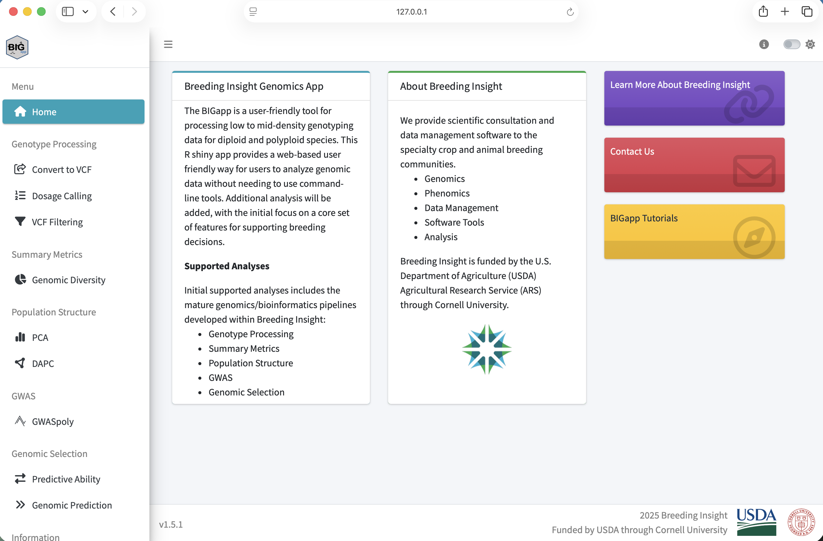
You should see the BIGapp welcome screen:
The Interface
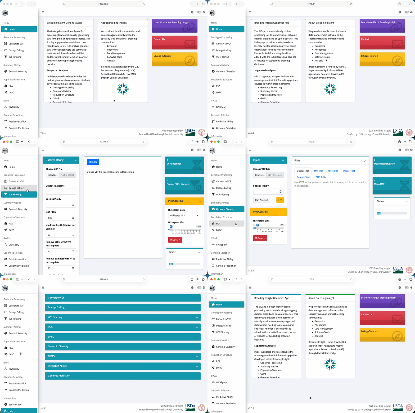
BIGapp is organized into sections in the left sidebar:
| Section | What it does |
|---|---|
| Dosage Calling | Convert raw read counts to genotype calls |
| Filtering | Quality control for SNPs and samples |
| Summary Stats | Calculate marker statistics (MAF, PIC, etc.) |
| PCA / DAPC | Visualize population structure |
| GWAS | Find marker-trait associations |
| Genomic Prediction | Predict breeding values |
Loading Data
What Data Do You Need?
At minimum, you need genotype data — a matrix showing which alleles each individual carries at each SNP.
| SNP1 | SNP2 | SNP3 | … | |
|---|---|---|---|---|
| Plant_001 | 0 | 1 | 2 | … |
| Plant_002 | 1 | 1 | 0 | … |
| Plant_003 | 2 | 0 | 1 | … |
The numbers represent dosage — how many copies of the alternate allele:
- 0 = homozygous reference (AA)
- 1 = heterozygous (AB)
- 2 = homozygous alternate (BB)
For polyploid crops (potato, blueberry, alfalfa, etc.), dosage can be higher: 0, 1, 2, 3, 4 for a tetraploid.
What is a VCF File?
VCF (Variant Call Format) is the standard file format for storing genetic variation data. When you get genotyping results back from a sequencing facility, they’re usually in VCF format.
A VCF file has two main parts:
1. Header lines (start with #) — metadata about the file:
##fileformat=VCFv4.2
##reference=Cmaxima_HZAU_T2T
##FORMAT=<ID=GT,Number=1,Type=String,Description="Genotype">
#CHROM  POS     ID      REF  ALT  QUAL  FILTER  INFO  FORMAT  Sample1  Sample2  Sample3
2. Data lines — one row per SNP, with genotypes for each sample:
Chr01 1234567 SNP_001 A G . PASS . GT:DP:AD 0/0:25:25,0 0/1:30:15,15 1/1:28:0,28The GT Field: Genotypes to Dosage
The GT (Genotype) field shows which alleles each sample has:
| GT Value | Meaning | Dosage |
|---|---|---|
0/0 |
Homozygous reference (e.g., AA) | 0 |
0/1 |
Heterozygous (e.g., AG) | 1 |
1/1 |
Homozygous alternate (e.g., GG) | 2 |
Remember the dosage table above? BIGapp converts VCF genotypes to dosage automatically. A 0/1 in the VCF becomes a 1 in the dosage matrix.
Other common FORMAT fields you might see:
- DP — Read depth (how many times this position was sequenced)
- AD — Allelic depth (reads supporting each allele, e.g.,
15,15means 15 reads for REF, 15 for ALT)
For this workshop, BIGapp handles the VCF parsing — you just upload the file!
How Data Loading Works in BIGapp
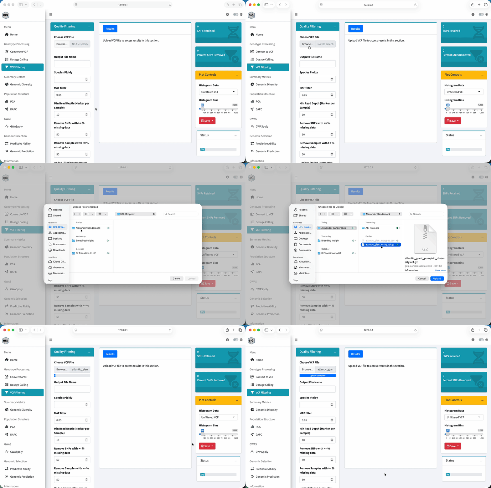
Unlike some tools with a central data loading area, each BIGapp module has its own file upload section. This means you’ll upload your VCF and phenotype files within each analysis module as needed.
Uploading a VCF File
When you open an analysis module (like VCF Filtering), you’ll see a “Choose VCF File” input:
- Click the “Browse…” button
- Select your VCF file from the file picker (
atlantic_giant_pumpkin_diversity.vcf.gz) - Click Open
- Wait for the “Upload complete” message to appear below the input
Uploading a Phenotype/Trait File
When you upload a phenotype CSV file, a Trait File Options modal will appear:
- Click “Browse…” next to the trait file input
- Select your phenotype CSV file (
atlantic_giant_pumpkin_diversity_phenotypes.csv) - Click Open
- In the modal that appears:
- Missing Data Value: Select how missing data is coded in your file (typically
NA) - Sample ID Column: Choose which column contains sample identifiers (select
Sample_ID) - Review the File Preview to verify your data looks correct
- Missing Data Value: Select how missing data is coded in your file (typically
- Click Save to confirm
The modal shows the first 5 rows of your data so you can verify the columns are being read correctly before proceeding.
Try It Yourself
Let’s practice by loading data in the VCF Filtering module:
- Go to VCF Filtering in the sidebar
- Upload the pumpkin VCF file using the steps above
- Verify you see “Upload complete”
Once you see “Upload complete” beneath the file input, your VCF is loaded and ready for filtering. The histogram on the right will populate once you run the filtering step.
Quality Control: Why It Matters
Raw genomic data almost always has problems:
- Bad markers — Some SNPs don’t amplify well or are in repetitive regions
- Bad samples — Some DNA extractions fail or get contaminated
- Missing data — Not every marker works for every sample
If we don’t filter these out, our downstream analyses will be unreliable.
Key Quality Metrics
For SNPs (markers):
| Metric | What it means | Typical filter |
|---|---|---|
| Call rate | % of samples with data for this SNP | Keep if > 80% |
| MAF | Minor allele frequency — how common is the rare allele? | Keep if > 5% |
| HWE | Hardy-Weinberg equilibrium test | Remove extreme deviations |
For Samples:
| Metric | What it means | Typical filter |
|---|---|---|
| Call rate | % of SNPs with data for this sample | Keep if > 80% |
| Heterozygosity | How heterozygous is this individual? | Remove outliers |
A SNP where 99% of individuals have the same allele doesn’t tell us much — there’s not enough variation to be useful for breeding decisions.
Demo: Filtering in BIGapp
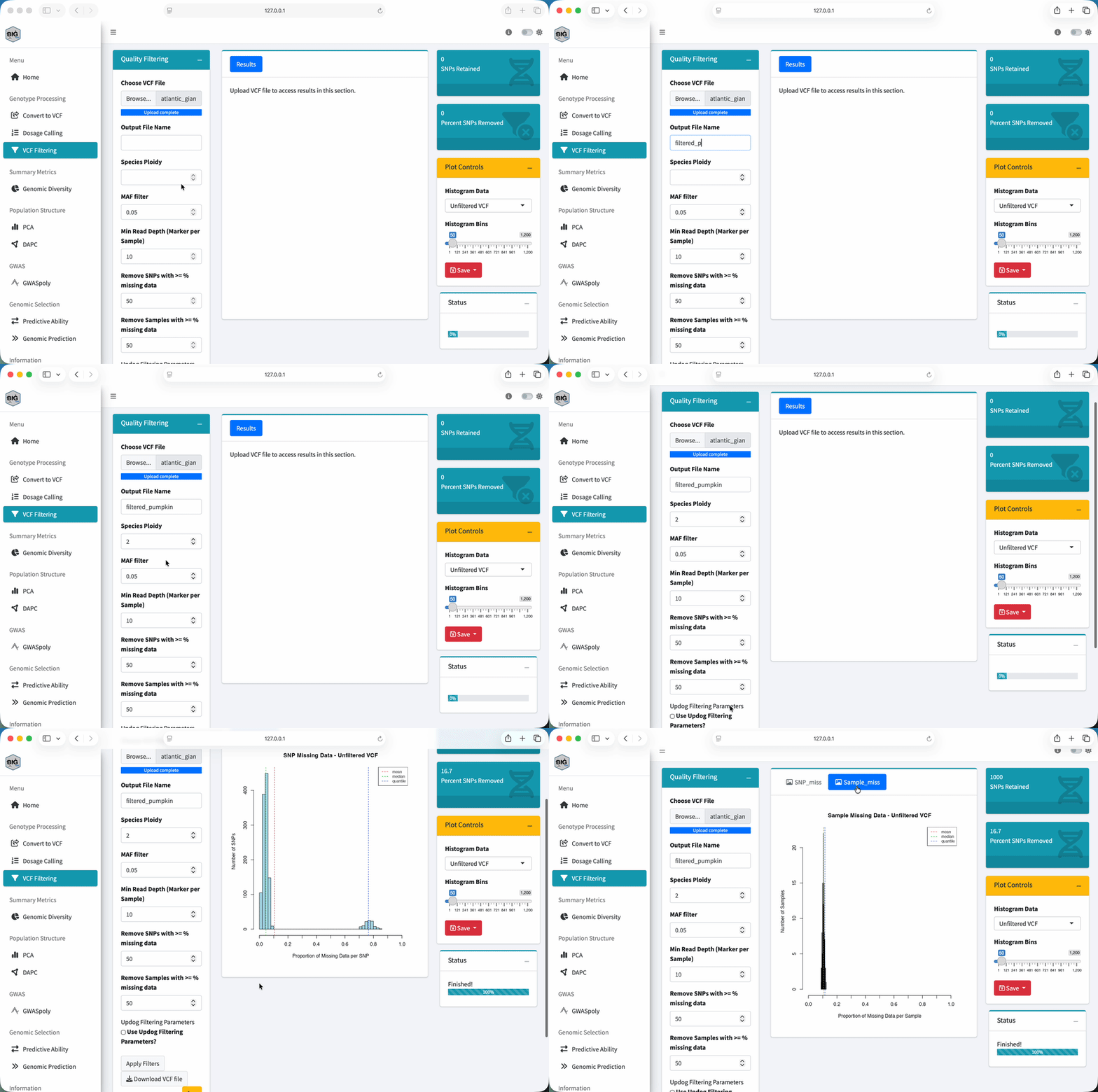
Watch how to apply quality filters:
Steps:
- Go to “SNP Filtering” in the sidebar
- Set Minimum MAF to 0.05 (5%)
- Set Maximum missing rate to 0.20 (20%)
- Click Apply Filters
- Note how many SNPs remain
Try It Yourself
- Apply MAF filter of 0.05
- Apply missing rate filter of 0.50 (50%)
- How many SNPs remain after filtering?
You should see the number of markers decrease from 1,200 to approximately 1,000. The pumpkin dataset includes ~100 low-MAF SNPs and ~100 high-missing SNPs specifically for this QC demonstration!
Summary Statistics
After filtering, let’s look at what we have.
Minor Allele Frequency Distribution
Go to Summary Stats → MAF Distribution
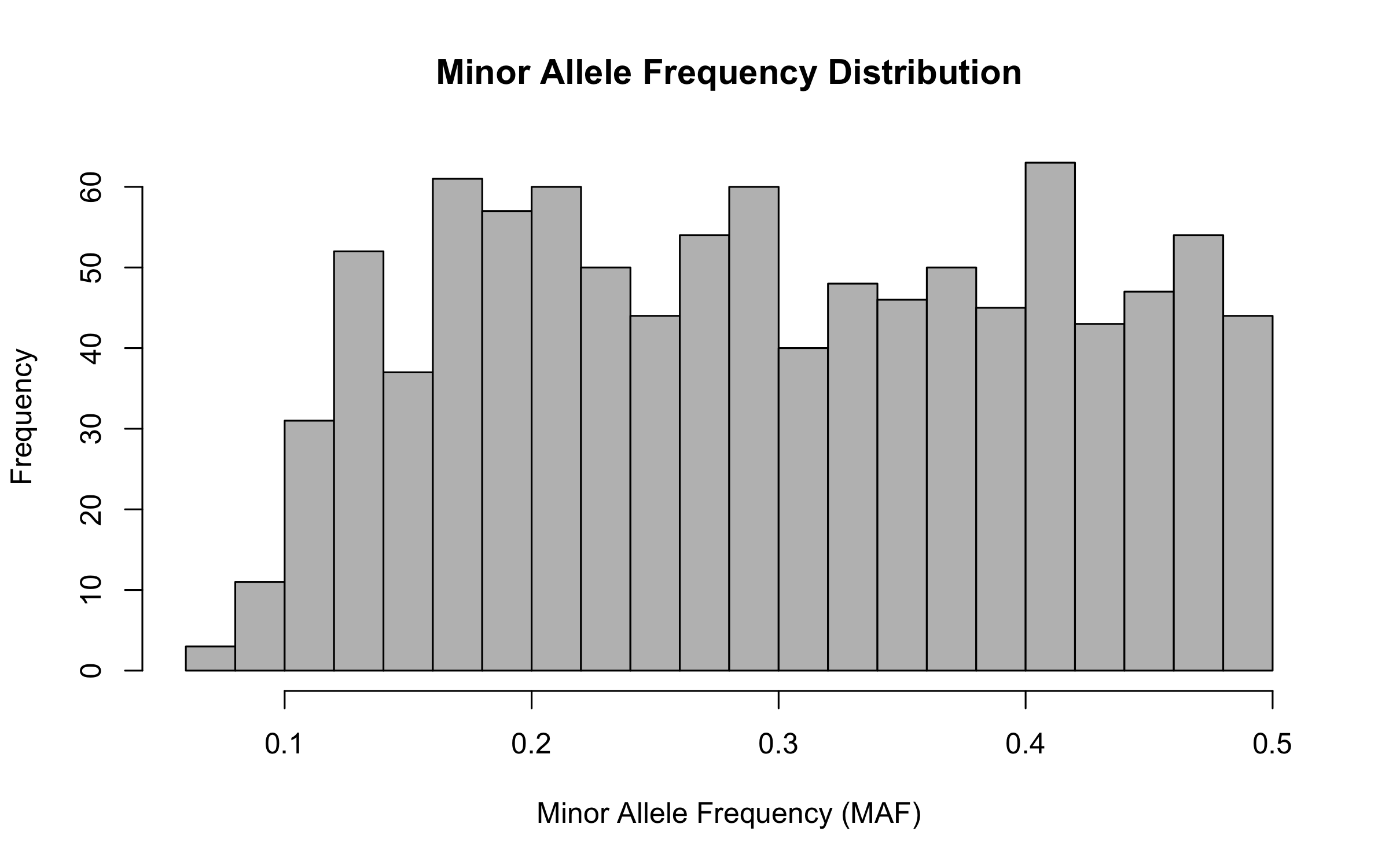
A healthy MAF distribution should be relatively flat — if it’s highly skewed toward low values, you may need stricter filtering.
Sample Heterozygosity
This shows how heterozygous each sample is. Look for:
- Outliers — Samples that are way more or less heterozygous than others might be mislabeled, contaminated, or have poor DNA quality
- Expected patterns — Inbred lines should be less heterozygous than F1 hybrids
Exercise
Using the pumpkin dataset:
- Load the VCF file
- Apply filters: MAF > 0.05, missing rate < 0.50
- Check the summary statistics
- Question: What percentage of markers were removed by filtering?
Starting with 1,200 markers, after filtering you should have ~1,000 remaining. That’s about 17% removed (200 ÷ 1,200 = 0.167).
Key Takeaways
✅ Genomic markers (SNPs) let us “see” genetic variation
✅ Quality control is essential — garbage in, garbage out
✅ Filter on MAF, call rate, and heterozygosity
✅ Check your data before running analyses
Next: Module 2: Population Structure & PCA — Understanding how your samples are related